Color Row Based On Cell Value Google Sheets - To format an entire row based on the value of one of the cells in that row: Select the range of rows you want. On your computer, open a spreadsheet in google sheets. To highlight a row based on a cell value, we need to use the “custom formula is” option in the conditional formatting menu. To apply conditional formatting to a whole row based on the value of one cell, follow these steps:
To apply conditional formatting to a whole row based on the value of one cell, follow these steps: Select the range of rows you want. On your computer, open a spreadsheet in google sheets. To format an entire row based on the value of one of the cells in that row: To highlight a row based on a cell value, we need to use the “custom formula is” option in the conditional formatting menu.
To apply conditional formatting to a whole row based on the value of one cell, follow these steps: To highlight a row based on a cell value, we need to use the “custom formula is” option in the conditional formatting menu. On your computer, open a spreadsheet in google sheets. To format an entire row based on the value of one of the cells in that row: Select the range of rows you want.

How to Change Cell Color in Google Sheets Based on Value MashTips
To highlight a row based on a cell value, we need to use the “custom formula is” option in the conditional formatting menu. Select the range of rows you want. To apply conditional formatting to a whole row based on the value of one cell, follow these steps: To format an entire row based on the value of one of.

Change Row Color Based on a Cell Value in Google Sheets
Select the range of rows you want. To highlight a row based on a cell value, we need to use the “custom formula is” option in the conditional formatting menu. To format an entire row based on the value of one of the cells in that row: To apply conditional formatting to a whole row based on the value of.
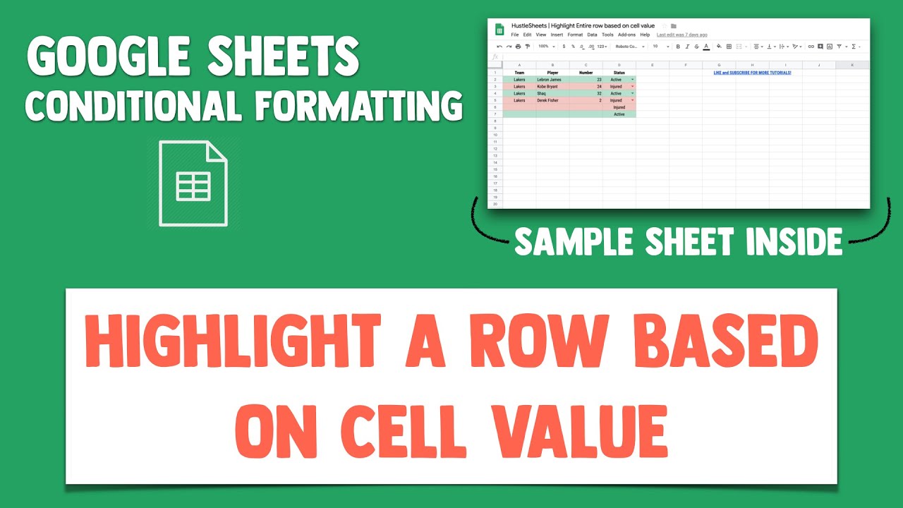
Highlight Entire Row a Color based on Cell Value Google Sheets
To highlight a row based on a cell value, we need to use the “custom formula is” option in the conditional formatting menu. On your computer, open a spreadsheet in google sheets. To apply conditional formatting to a whole row based on the value of one cell, follow these steps: To format an entire row based on the value of.

Change Row Color Based on a Cell Value in Google Sheets
On your computer, open a spreadsheet in google sheets. Select the range of rows you want. To format an entire row based on the value of one of the cells in that row: To highlight a row based on a cell value, we need to use the “custom formula is” option in the conditional formatting menu. To apply conditional formatting.

Change Row Color Based on a Cell Value in Google Sheets
Select the range of rows you want. To highlight a row based on a cell value, we need to use the “custom formula is” option in the conditional formatting menu. To apply conditional formatting to a whole row based on the value of one cell, follow these steps: To format an entire row based on the value of one of.

Change Row Color Based on a Cell Value in Google Sheets
Select the range of rows you want. To format an entire row based on the value of one of the cells in that row: On your computer, open a spreadsheet in google sheets. To highlight a row based on a cell value, we need to use the “custom formula is” option in the conditional formatting menu. To apply conditional formatting.

Change Row Color Based on a Cell Value in Google Sheets
To highlight a row based on a cell value, we need to use the “custom formula is” option in the conditional formatting menu. On your computer, open a spreadsheet in google sheets. Select the range of rows you want. To format an entire row based on the value of one of the cells in that row: To apply conditional formatting.

Change Row Color Based on a Cell Value in Google Sheets
To apply conditional formatting to a whole row based on the value of one cell, follow these steps: On your computer, open a spreadsheet in google sheets. To highlight a row based on a cell value, we need to use the “custom formula is” option in the conditional formatting menu. To format an entire row based on the value of.
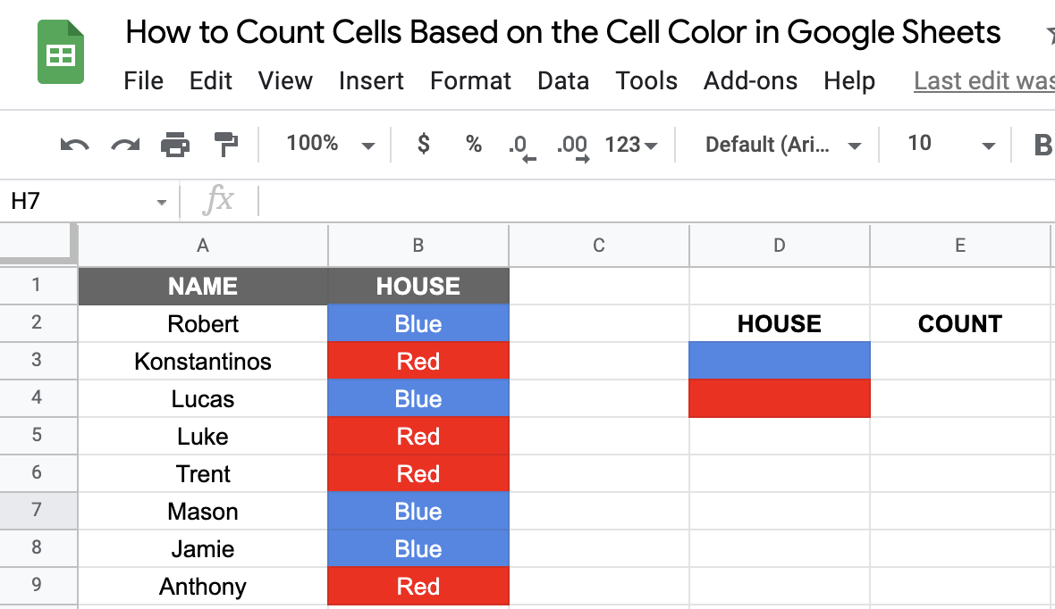
count cells based on cell color google sheets
To highlight a row based on a cell value, we need to use the “custom formula is” option in the conditional formatting menu. To format an entire row based on the value of one of the cells in that row: On your computer, open a spreadsheet in google sheets. Select the range of rows you want. To apply conditional formatting.

count cells based on cell color google sheets
On your computer, open a spreadsheet in google sheets. To format an entire row based on the value of one of the cells in that row: Select the range of rows you want. To highlight a row based on a cell value, we need to use the “custom formula is” option in the conditional formatting menu. To apply conditional formatting.
To Highlight A Row Based On A Cell Value, We Need To Use The “Custom Formula Is” Option In The Conditional Formatting Menu.
Select the range of rows you want. To apply conditional formatting to a whole row based on the value of one cell, follow these steps: To format an entire row based on the value of one of the cells in that row: On your computer, open a spreadsheet in google sheets.